
Ethiopian Economics Association
The Ethiopian Economics Association (EEA) was established as a non-profit making, non-political and non-religious..
Recent news
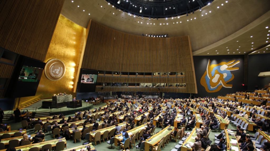
The Seventeenth International Conference on the Ethiopian Economy
The Seventeenth International Conference on the Ethiopian Economy was organized by the Ethiopian Economics Association (EEA) on July 18-20, 2019 in the organization’s Conference Hall, Addis Ababa Ethiopia. The conference was co-organized by the Ethiopian Strategy Support Program (ESSP II) of the International Food Policy Research Institute. The conference was able to…

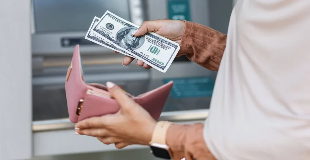
The Pros and Cons of Unsecured Loans
Unsecured loans are the ones that do not require any collateral. In contrast, a secured loan uses your property, a valuable object, or an auto title to guarantee loan repayment. The question here is whether it is worth borrowing money through an unsecured loan. Financial experts state that the choice depends on each case. Borrowers have two…
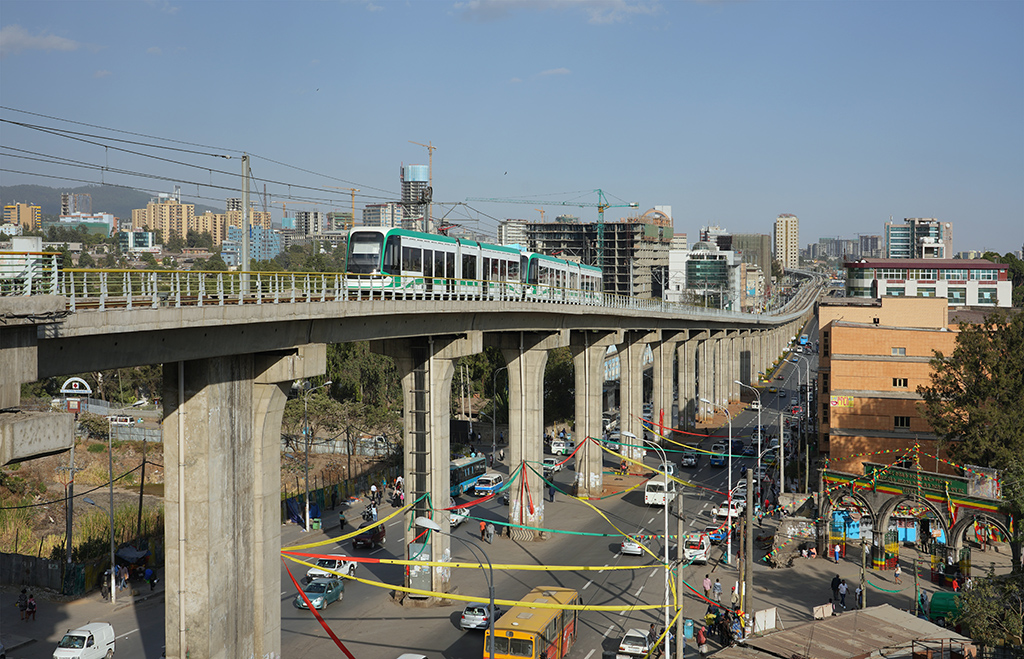
July 18-20: 17th International Conference on the Ethiopian Economy (Addis Ababa, Ethiopia)
On July 18-20, 2019 the Ethiopian Economics Association Collaborative will host its 17th International Conference in Addis Ababa, Ethiopia.
This year, the conference will focus on Macroeconomic Instability and Agenda for Reform in Ethiopia, agriculture, social Welfare, Trade and Financial Liberalization, Monetary and Fiscal Policies for sustainable development, labor markets…
How Online Payday Loans Work
Everybody has heard about payday lenders offering loan options for people who need money urgently. An increasing number of businesses provide lending services, and a growing number…
Do $400 Loans Are a Good Solution in Any Situation?
$400 loans are the type of borrowings that people usually take when facing financial difficulties. We all can get into a situation when we need to repair a car, pay for our medical bills, or cover current needs in case of personal reduction or salary cuts. Payday loans from direct lenders can become your financial assistance in all the financial emergencies or unexpected expenses you may face…
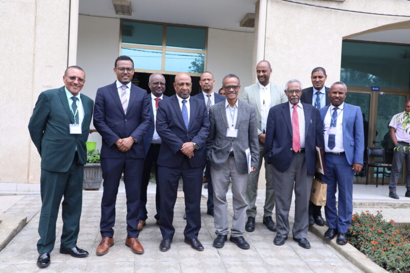
25th General Assembly of EEA 2018
The 25th General Assembly(GA) meeting was held on November 17, 2018 at EEA head office in Addis Ababa, Ethiopia. The general assembly meets once a year to present and discuss the work that has been done in the fiscal year(2017/18), endorsed external auditors report and approve the plan for the next year(2018/19). The meeting was attended by EEA members and invited stakeholders.
Do Cash Advances Hurt Your Credit Score?
A cash advance is a sum of money that people borrow in case of financial emergencies. They then repay their debt with interest when getting their next paycheck. Ideal for emergency purchases, cash advances are easy to get. Do these loans hurt your credit score? The short answer is usually no.
16th International Conference on the Ethiopian Economy
The 16th International Conference on the Ethiopian Economy was held from July 19-21, 2018 at the Ethiopian Economics Association(EEA) conference hall. The Ethiopian strategic support program (ESSP) of the collaborative program of International Food Policy Research Institute (IFPRI) and the Ethiopian Development Research institute co-organized the conference with EEA.
Announcements
- 17th International Conference on the Ethiopian Economy Papers and Abstracts
- The Ninth Annual Conference on the Southern Nations and Nationalities Peoples Regional State Economic Development
- Debt accumulation, its sustainability and impact on Ethiopia’s Economy
- Draft Papers Presented On The 16th International Conference On Ethiopian Economy
- Call for Papers for 7th Eastern Ethiopia Conference
- Call for Papers 6th Tigray Regional Conference 2018
- Call for papers for a Special Issue on “Gender and Industrialization in Ethiopia” in the Ethiopian Journal of Economics (EJE)
Our projects
- Revenue potential study in Afar Regional State
- Revenue potential study in Southern Nations Nationalities and People Regional State
- Price Volatility and Food Security
Recent publications
- PROCEEDINGS OF THE SIXTH ANNUAL CONFERENCE ON THE EASTERN ETHIOPIA ECONOMIC DEVELOPMENT :V. No. –
- Report on the Ethiopian Economy 2018 :V. No. –
- Report on the Ethiopian Economy 2017 :V. No. –
- Report on the Ethiopian Economy 2016 :V. No. –
- Ethiopian Journal of Economics :V. XXVII No. 1- April 2018
- Ethiopian Journal Of Economics :V. XXVII No. 1- April 2018
Related links
©2024 Ethiopian Economic Association